CSET Math Practice Test and Prep

Welcome to our CSET Mathematics practice test and prep page. On this page, we outline the domains and key concepts for the CSET Mathematics exam. It is a free resource we provide so you can see how prepared you are to take the official exam.

While this free guide outlines the domains found on the exam, our paid CSET Mathematics study guide covers EVERY concept you need to know and is set up to ensure your success! Our online CSET Mathematics study guide provides test-aligned study material using interactive aids, videos, flash cards, quizzes and practice tests.

Will I pass using this free article? Will I pass using your paid study guide?

If you use this guide and research the key concepts on the CSET Mathematics exam on your own, it’s possible you will pass, but why take that chance? With our paid study guide, we guarantee you will pass.

→ Subscribe Now: CSET Mathematics

Not ready to start studying yet? That’s OK. Keep reading, and when you’re ready, take our free CSET Mathematics practice tests.

In this article, we will cover:

 

• CSET Math Test Information
• CSET Math Subtest I
• CSET Math Subtest II
• CSET Math Subtest III

CSET Math Test Information

Subtest I tests Number and Quantity and Algebra. Subtest II tests Geometry and Probability and Statistics. Subtest III tests Calculus. For the Single Subject Teaching Credential in Mathematics, you must pass Subtests I, II, and III. This credential authorizes the teaching of all mathematics coursework.

Cost:

$99 per subtest

Scoring:

220 (out of 300) per subtest

Pass rate:

According to the CTC Annual Passing Rate Report, the CSET Mathematics test had a 61.2% passing rate for 2019-2020.

Study time:

It is recommended to study 30 to 45 minutes a day until you feel confident with the majority of these topics.

What test takers wish they would’ve known:

• A graphing calculator will be allowed for Subtest II only, you must bring an approved calculator with you.
• Test results take up to 7 weeks.
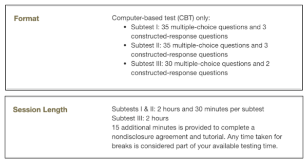
• Any time taken for breaks is considered part of your testing time.
• There are 2-3 constructed-response questions on each subtest.

Information and screenshots obtained from the California Educator Credentialing Assessments website: https://www.ctcexams.nesinc.com/Home.aspx

CSET Math Subtest I

Overview

Subtest I has 35 multiple-choice questions and 3 constructed-response questions. You will have 2.5 hours to complete this subtest.

There are two domains, both with specific competencies:

• Number and Quantity
• The Real and Complex Number Systems
• Number Theory
• Algebra
• Algebraic Structures
• Polynomial Equations and Inequalities
• Functions
• Linear Algebra

Number and Quantity: The Real and Complex Number Systems

This section tests your knowledge on performing operations and solving problems involving the real and complex number systems.

Let’s discuss some concepts that will more than likely appear on the test.

Subsets of the Real Number System

Integers are the set of real numbers with no fractional part. Examples:

-3, -7, 0, 5, 21

Rational numbers are real numbers that can be formed by dividing two integers. They can be written in either fractional or decimal form. When written in decimal form, a rational number either terminates or repeats forever. Examples:

4/9, -(6/4), 2, 1.25, -6.6, 3.3

3

Irrational numbers are real numbers that cannot be formed by dividing two integers. Irrational numbers include decimals that go on forever without repeating.

For example, the special number π (pi) is an irrational number.

Properties of Subsets of the Real Numbers

The following properties hold true for all real numbers a, b, and c:

The Associative Property of Addition states that ( a + b ) + c = a + ( b + c ). Similarly, the Associative Property of Multiplication

states that ( ab ) c = a ( bc ).

For example:

(4 + 5) – 6 = 4 + (5 – 6) = 3

(-1 ∙ 3)4 = -1(3 ∙ 4) = -12

The Commutative Property of Addition

states that a + b = b + a .

Multiplication of real numbers is also commutative since ab = ba .

Note that division is not commutative since

a/b ≠ b/a

not associative since ( a ÷ b ) ÷ c ≠ a ÷ ( b ÷ c ).

The Additive Identity Property

states that a + 0 = a , where 0 is the additive identity. For example:

-9 + 0 = -9

The real number 1 is the Multiplicative Identity

since a ∙ 1 = a for all real numbers. For example:

7∙ 1 = 7

The Distributive Property

states that a ( b + c ) = ab + ac . For example:

-2(3 + 6) = -2(3) + -2(6)

The set of real numbers is said to be closed

under addition and multiplication because performing these operations always gives a real number back.

The set of real numbers is not closed under division, because dividing two real numbers does not always produce a real number. When dividing by zero, the result does not exist.

Number and Quantity: Number Theory

This section tests your knowledge on the properties of natural numbers, number theory facts, and the Euclidean Algorithm.

Here are some concepts that you may see on the test.

Properties of Divisibility

For real numbers, a , b , and c, the following are true:

• If a nonzero integer divides two other integers, then it divides their sum.

For example:

3 divides 9 evenly, and 3 divides 6 evenly. Applying this property means that

3 divides 9 + 6. In fact, 3 does divide 15 since 15 divided by 3 is 5.

• Ifa divides b, and b divides c, then a divides c , where a , b , and c are nonzero integers.

For example:

2 divides 4, and 4 divides -16. Applying this property means that 2 divides -16,

which it does since -16 divided by 2 is -8, an integer.

• Ifa divides b then a divides a scalar multiple of b .

For example:

5 divides 20. Applying this property then means that 5 divides any scalar multiple of 20, which it does. For example, 5 divides -40 which is -2(20), since -40 divided by 5 is -8.

Euclidean Algorithm

The Euclidean Algorithm is a method for finding the greatest common divisor for two integers.

For integers a and b, where a ≥ b , the greatest common divisor (gcd) is given by the following:

1. Ifb = 0, then gcd( a , b ) = a .
2. Ifb > 0, then gcd( a , b ) = gcd( b , r ) where r is the remainder of a divided by b.

For example, let’s find the greatest common divisor of 8,602 and 4,278. Here, a = 8602 and b = 4278. Since 4278 > 0, we need to use the second part of the algorithm and find the remainder of 8602 divided by 4278. 4278 goes into 8602 two times with a remainder of 46.

Therefore, gcd(8602, 4278) = gcd(4278, 46). Now we can apply the algorithm again with these new smaller numbers. 46 goes into 4278 ninety-three times with a remainder of 0.

Therefore, gcd(4278, 46) = gcd(46, 0). Using the first part of the algorithm, we know that gcd(46, 0) = 46.

Putting this all together, gcd(8602, 4278) = gcd(4278, 46) = gcd(46, 0) = 46. So, the greatest common divisor of 8,602 and 4,278 is 46.

Algebra: Algebraic Structures

This section tests your knowledge on solving algebraic equations and inequalities, as well as fields and rings.

Let’s look at some concepts that are guaranteed to come up on the test.

Factoring

Factoring is writing a polynomial as the product of two other polynomials. This is usually applied to simplify an expression involving polynomials or to find the roots of a polynomial. There are many strategies for factoring polynomials, including factoring out the greatest common multiple, factoring perfect square trinomials, factoring by grouping, etc. Below are some examples of polynomials and their factors:

x² + 5 x + 6 = ( x + 2)( x + 3)

x² – 144 = ( x – 12)( x + 12)

4 x³ – 8 x = 4 x ( x² – 2)

Since this is a broad topic, we will not discuss all the factoring methods here, but this is something you should study on your own.

Equivalent Expressions

Expressions are equivalent if, when you assign a non-zero number to the variable, the expressions are equal.

For example, 8 x – 9 is equivalent to (

2(16x-18))/4. You can determine this by substituting x = 1 into the expressions. 8 x – 9 is -1 when x = 1, and (

2(16x-18)/4) is also equal to -1 when x = 1.

7 x² – 3 is not equivalent to ( x + 2)(7 x + 3); you can check by substituting x = 0 into the expression:

7(0)²

– 3 = -3, but (0 + 2)(0 + 3) = 6.

Algebra: Polynomial Equations and Inequalities

This section tests your knowledge on finding the roots of polynomial equations and the solutions of polynomial inequalities.

Here are some specific concepts that will more than likely appear on the test.

The Factor Theorem

The Factor Theorem states that for a polynomial f ( x ), f ( c ) = 0 if and only if x – c is

a factor of f ( x ).

This means that if c is a root of the polynomial, then x – c is a factor of the polynomial, and if x – c is a factor of the polynomial, then c is a root.

This is often used to help factor polynomials or to find the roots of a polynomial. If we already know one root of a polynomial, we can use long division of polynomials to find the other roots.

For example:

( x – 8) and ( x + 1) are factors of the polynomial f ( x ) = x²

– 7 x – 8. According to the theorem, this means that x = 8 and x = -1 are roots of the polynomial. To check this, compute f (8) = 8²

– 7(8) – 8 = 0 and f (-1) = (-1)²

– 7(-1) – 8 = 0.

The Binomial Theorem

Algebra: Functions

This section tests your knowledge on function families, their graphs and properties, and performing operations on functions.

Let’s discuss some concepts that will more than likely appear on the test.

Logarithmic Functions

A logarithmic function is the inverse of an exponential function.

y=log_bx

is the logarithmic function of base b.

This equation can be rewritten in exponential form as

b^y=x

You can identify the standard logarithmic function from its graph by the following characteristics:

• x-intercept at the point (0, 1) and has noy -intercept
• The graph has a vertical asymptote at the linex= 0
• Ifb> 1, the function is increasing, and if 0 < b < 1, the function is decreasing
• The function is continuous

Inverses

Functions f and g are called inverse functions if f ( g ( x )) = x for all values in the domain of f and g ( f ( x )) = x for all values in the domain of g . The inverse of f can be written as f -1. The domain of f is the range of f -1, and the range of f is the domain of f -1.

For example, f ( x ) = 5 x – 2 and g ( x ) =x+2/5 are inverse functions which we can check by computing f ( g ( x )) = 5(x+2/5)– 2 = (x + 2)– 2 = x and g ( f ( x )) = ((5x-2) + 2)/5= x.

The graphs of inverse functions are reflections of each other over the line y = x . For example, f ( x ) = x 2+ 3 and g ( x ) = x-3

are inverse functions as you can see from the graph below:

Algebra: Linear Algebra

This section tests your knowledge on lines, vectors, and systems of linear equations.

Here are some concepts that you may see on the test.

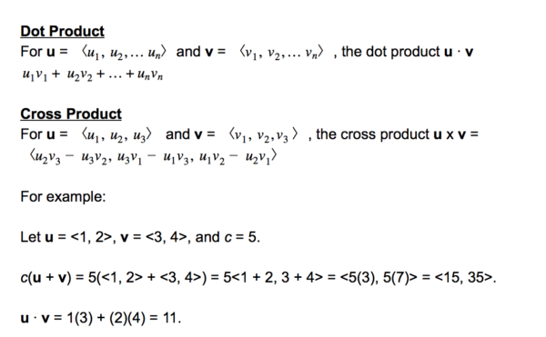
Basic Properties of Vectors

Addition and scalar multiplication of vectors work like you would expect them to, since they follow the same properties as real numbers. If u, v, and w are vectors, and c and d are scalars, then we can say the following:

However, instead of simply being able to multiply vectors, there are two different special operations.

Linear Equations

A linear equation is the equation of a line, where the variable is degree 1 and can be written in the form y = mx + b, where m is the slope of the line and b is the y -intercept.

For example, y = -2 x – 9 and 9 x – 8 = 3 are linear equations.

And that’s some basic info about CSET Math Subtest I.

CSET Math Subtest II

Overview

Subtest II has 35 multiple-choice questions and 3 constructed-response questions.

There are two domains, both with specific competencies:

• Geometry
  • Plane Euclidean Geometry
  • Coordinate Geometry
  • Three-Dimensional Geometry
  • Transformational Geometry
• Probability and Statistics
  • Probability
  • Statistics

This section tests your knowledge of geometric concepts related to the Euclidean plane, which is just a flat, two-dimensional “area” with no coordinates or any other defining characteristics. The simplest concrete example of a Euclidean plane is a plain sheet of paper. It is named after the mathematician Euclid, who outlined many of the facts (which he called axioms and postulates) related to points, line segments, rays, lines, angles, and other figures which can be constructed in the plane. Euclidean geometry can be done with only a straightedge and compass, and all of Euclid’s work in his book,

The Elements is based on constructing figures using just these two tools.

Let’s take a look at some of the common elements found in plane Euclidean geometry.

Points

The most basic unit of structure found in plane Euclidean geometry is the point.  It is a single dot, usually used either to indicate a part or to build, some other figure. In geometry, we name things by the points that make them, so the point in the example below would be called point A.

Line Segments, Rays, and Lines

Line segments, rays, and lines are all defined by a pair of points in the Euclidean plane.

Let’s start simply. If you draw two points on a sheet of paper and connect them with a straightedge, without going past the points, you have created a line segment. Defined simply as a line connecting two points, this is the simplest linear form in geometry.  Lines, rays, and segments are all named by the two points that define them. Pictured below is line segment AB:

In order to draw a ray, begin with two points, draw a line from one point to the other, and then keep going. A ray begins at one point, passes through another, and then keeps going forever. This is denoted by placing an arrow point on one end of the ray. Pictured here is ray AB:

Finally, let’s draw a line. Just like with a line segment or ray, begin with two points. Then, draw a line that passes through both of them but keeps going on both sides – forever! This is denoted by placing arrow points at both ends of the line. Pictured here is line AB:

Angles

You can think of geometry, and a lot of math really, like a ladder. Each concept builds on the concepts before it. We started with a point, the most basic element in geometry. By adding a second point, we can create a line. Now, by creating a second line, we can create an angle.

To understand angles, let’s make one. First, draw a line by connecting two points and extending past them. Now, draw a second line that intersects the first one. A pair of lines, as long as they intersect, will always intersect at a point. We call this point the vertex, and at that point they make angles. Angles are named by their parts, with the vertex always in the middle. For example, pictured below are lines AB and CE, which intersect at point D :

The indicated angle is angle ADC. Since the vertex is D, it is in the middle of the angle’s name. Sometimes, you may see this denoted with an angle symbol: ∠. For example, ∠ADC.

An angle that looks like a plain straight line is called a straight angle and measures 180 degrees. In the example above, the angle ADB is a straight angle.

An angle that looks like a square corner is called a right angle and has a measure of 90 degrees. An angle that is smaller than a right angle is called acute, and an angle that is larger than a right angle (but smaller than a straight angle) is called obtuse. In the example, angle ADC is acute, and angle ADE is obtuse. We denote right angles with a square indicator, instead of a curved one. See the right angle FGH in the example below:

Two lines that intersect at right angles are called perpendicular, and two lines that never, ever intersect are called parallel (you can remember this, because the two L’s in the middle of “parallel” form parallel lines).

Geometry: Coordinate Geometry

So, let’s start with Plane Euclidean Geometry.

Geometry: Plane Euclidean Geometry

In-plane Euclidean geometry, we study points, lines, figures, and some of the relationships between those components; however, to get a little deeper understanding of those relationships, as well as discover some new ones, it is helpful to add some context. That is where coordinate geometry comes in.

Coordinate geometry is done on the coordinate plane, also known as the Cartesian plane. The coordinate plane is made up of two

axes (axes is the plural of axis), called the x-axis (horizontal) and the y-axis (vertical). Now, by using a system of ordered pairs of x and y coordinates, we cannot only draw points, lines, and figures, but we can determine their locations.

An ordered pair is like a set of instructions on how to get to a point on the coordinate plane. It looks like a pair of numbers – for example, (1,5); (3,0); (-5,1). These ordered pairs explain the location of a point in terms of the axes – (x,y) – first x, then y. You can think of it like getting directions from your navigation app: first, go this far along the x-axis, and then go this far along the y-axis.

When using ordered pairs, we always begin at the origin – the point (0,0), where the two axes meet. In the coordinate plane, the x-axis is positive toward the right and negative toward the left. Similarly, up is positive on the y-axis and down is negative. So, in order to plot the point (1,5), we will begin at the origin, go 1 to the right on the x-axis, and then go up 5.

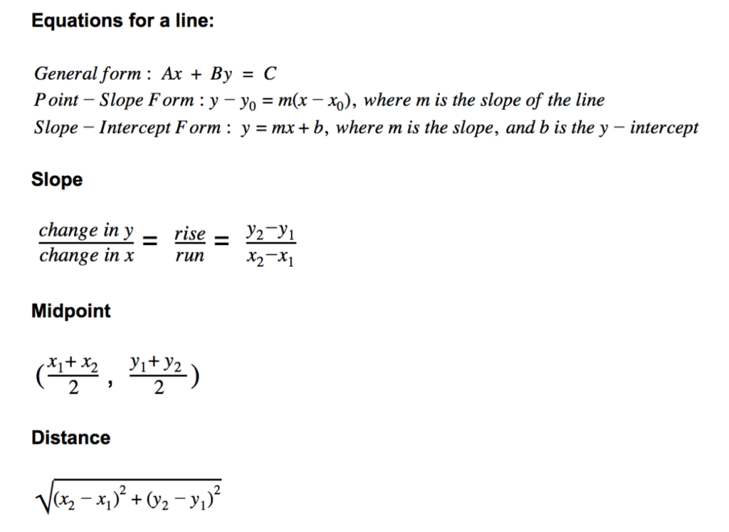
In coordinate geometry, we have some important formulas to help us determine lines in the plane, the slope of a line, the midpoint of a line, and the distance from one point to another. They are:

Geometry: Three-Dimensional Geometry

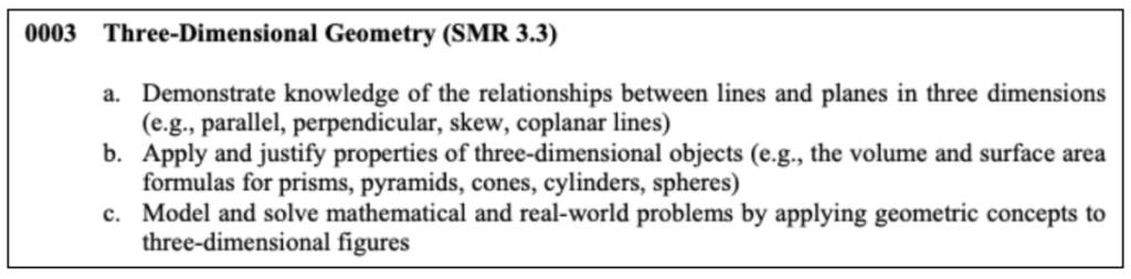
Three-dimensional geometry is, as the name would suggest, the mathematics of shapes and objects in three dimensions. It involves shapes like cubes, cuboids, and polyhedrons; 3D geometry is all about objects that have height, width, and depth. Just like 2D geometry can be done on a plane, which has two dimensions, 3D geometry adds a z-axis to the plane. You can visualize the z-axis as going through your screen or a sheet of paper when you look at a Cartesian plane. This is called a space, and in the case of three dimensions, it’s called a 3-space.

Shapes in three dimensions are called geometric solids.

They include:

• Cube: a solid whose faces are square.
• Cuboid: a solid whose faces are rectangular.
• Square Pyramid: a solid with a square shaped bottom and four triangular sides.
• Triangular Pyramid: a solid whose faces are all triangles.
• Cone: a solid with a circular face at the bottom and a single point at the top, called the apex; every line segment connects the apex to a point on the circle.
• Cylinder: a solid with circular faces connected by a curved surface.
• Sphere: a solid defined by a central point P and every point in three dimensions at a distance R from P; it looks like a ball.

Many 2D shapes have 3D solid analogs. For instance, a sphere is the 3D analog of a circle. We understand what these shapes look like, and thanks to geometry, we can describe them by simply extending plane geometry slightly.

In two dimensions, the parallel postulate tells us that when given a point A and a line BC which does not contain A, there exists one and only one line passing through A that does not intersect BC. This is not true in three dimensions! Once we add the third dimension, the z-axis, you can create all sorts of lines coming from outside the plane (or above the sheet of paper) that will pass through A but never intersect BC.

These lines are called skew lines. They are not parallel since they don’t exist in the same plane, but they never intersect, and there are infinitely many such skew lines for any line BC and point A.

Now, suppose I want to draw a line perpendicular to line BC. I can draw one in the plane that intersects it at point D, but in three-dimensional space, I can draw any number of lines passing through D which form a right angle with line AB. What does this mean? In the realm of 3D geometry, there are infinitely many lines that are perpendicular to a given line.

In 3D space, we cannot only draw lines, but we can also have entire planes next to each other, and just like lines, those planes can sometimes intersect. Two planes that intersect at right angles are perpendicular, and two planes that never intersect are parallel. The same parallel postulate holds for planes – given a plane A and a point B not on A, there is one and only one plane passing through B which never intersects A.

Let’s talk about another concept that is likely to appear on the test.

Planar Sections

Another major topic in 3D geometry is the concept of cross-sections. If you’ve ever enjoyed sliced cheese or a sandwich, or if you’ve opened a dollhouse to see the rooms inside, you’re familiar with the concept of a planar section. The slicing knife and the line where the dollhouse opens represent the “plane” in this case. By taking planar cuts of geometric solids, you can produce two-dimensional shapes. Here are a few examples of planar sections:

The image above depicts a sphere with a planar cut through it. Notice that the planar cut of this sphere produces a circle. In fact, no matter how you cut a sphere, the resulting shape will always be a circle; however, this isn’t always the case for other solids.

For example, take a look at this square pyramid above. We’ve taken four plane sections from it, and each one produces a different shape. Depending upon where you cut the pyramid, your planar section could be a square, a trapezoid, or a triangle.

Geometry: Transformational Geometry

Transformational geometry is the study of transforming shapes by means of various operations:

• Translation: Moving a shape without changing its orientation, like sliding a puck across the ice.
• Rotation: Turning a shape around a point, like spinning a record.
• Reflection: “Flipping” a shape over, like flipping a pancake.
• Dilation: Making a shape larger or smaller (but preserving proportions), like enlarging something in a magnifying glass.

Two shapes are said to be congruent if one can be obtained from the other by translation, reflection, and rotation. Two shapes are said to be similar if one can be obtained from the other by translation, reflection, rotation, and dilation.

The factor by which the length of every side of a dilated figure differs from the original is called the scale factor. For example, if the original figure contains a side AB, a similar figure will contain a side of length rAB, and the scale factor would be called r.

Geometry: Probability

Probability is the study of how likely an event is to occur. In probability terms, the word event refers to any outcome of a trial or experiment. For example, if you flip a coin, the coin landing on heads is one event, and the coin landing on tails is another. The probability of either event, for a single coin flip, is 50%, or 0.5.

The probability of an event is often expressed as a fraction or decimal. For an event A , we say that the probability that A will occur is P(A) , and P(A) is a number somewhere between 0 and 1, inclusive. An event with a probability of 0 is impossible – it will never occur. For example, the probability of rolling a 7 on a single six-sided die is 0. On the other hand, an event with a probability of 1, corresponding to 100%, is certain. On a regular coin, the probability of flipping either tails or heads is 100% – you’re guaranteed to get one or the other.

In the study of probability, it is important to think about how many outcomes are possible. For a given experiment, the set of all possible outcomes is called the sample space. For example, for rolling a single six-sided die, the possible outcomes are all the numbers from one to six, so the sample space for this experiment is S = {1,2,3,4,5,6}. The number of elements in the sample space is the number of possible outcomes in an experiment.

So, using this information, you can express the probability of a given outcome with the following ratio:

So, on a single six-sided die, what is the probability of rolling a 3? There is one way to roll a 3 and six possible outcomes, so P(3) = ⅙.

In this example, the probability for each outcome in the sample space is the same – ⅙. Think about this: What do you get if you add up all of the probabilities in the sample space? In this case, ⅙ + ⅙ + ⅙ + ⅙ + ⅙ + ⅙ = 1.

That’s not a coincidence. The probability distribution – that is, the set of all probabilities – for a sample space will always sum to one. This is true even if the probabilities within the sample space are different.

Let’s discuss a couple of concepts that will more than likely appear on the test.

Addition Rule for Disjoint Events

Think about rolling a six-sided die again. Is it possible to roll a four and a six at the same time? Not on a single die, it isn’t. These events are said to be mutually exclusive , which is also called disjoint. Here are some examples and nonexamples of disjoint events:

• Rolling a one or a three on a single six-sided die: DISJOINT.
• Rolling a two or rolling an even number: NOT DISJOINT (two is an even number, so if you roll a two, you’ve done both).
• Drawing a king or a queen from a deck of cards: DISJOINT.
• Drawing a king or drawing a heart: NOT DISJOINT (you may draw the king of hearts).

When two events are disjoint, we sometimes think about the probability of one thing or the other happening. The key word in this phrase is the word “OR.”

The probability that A or

B occurs is the sum of their individual probabilities:

P(A or B) = P(A) + P(B)

For example, suppose you spin a wheel to try to win a prize. There are 100 total slots on the wheel: 1 of those is green and wins a grand prize, 10 are yellow and win a second prize, 20 are blue and win a small prize, and the rest of the spaces are black and result in no win. What is the probability that you win the grand prize or a second prize?

P(Grand Prize OR Second Prize) = P(Grand Prize) + P(Second Prize)

= 1/100 + 10/100

= 11/100

= 0.11

Geometry: Statistics

Statistics is the study of data and how that data “looks.” A set of data points forms a “distribution” of that data, which can be visualized one of many ways including in histograms, stem and leaf plots, box plots, or two-way tables. One of the most basic concepts in statistics is the concept of the center of a distribution.

Center

The three measures of center are mean, median, and mode. The mean of a distribution is the sum of all data points, divided by n , the number of data points. This is also known as the average.

The median of a distribution is the value in the “middle” – as many above as below. In the case that n is even – that is, there are an even number of data points – there will not be a single value in the middle, but two. The average of these two data points is the median.

While mean and median are common measures of center, it is sometimes difficult to know which is better. The answer to this question is the concept of resistance. Suppose we poll a city block, asking each household their annual income. Suppose this block is mostly middle-class families making about $50,000 per year and one NBA superstar who makes millions. What do you think that NBA star will do to the mean? It will make it much higher than the average income for the rest of the families on the block; however, since the median doesn’t care how large or small the values above it may be, it is more or less unaffected by the extremely high income.

For this reason, we say that the median is resistant to outliers. An outlier is a data point that lies far outside the rest – it’s an oddball! If you suspect outliers in your data set, it is usually better to use the median than the mean.

The mode of a distribution is the value that appears most often in a set of data points. While mean and median deal with quantitative values – numbers, in other words – the mode is usually used in the case of categorical values. For example, if a survey asks, “what is your favorite flavor of ice cream?” it is not possible to find a mean or median for these responses – it is, however, possible to determine which flavor was mentioned most often, and that flavor is called the mode.

The Normal Distribution

The normal distribution is one of the most important concepts in statistics. It describes a distribution that is unimodal, meaning when you graph it in a histogram, it only has one “hump” and is symmetric and bell-shaped. This is a depiction of the normal distribution:

The normal distribution is centered at the mean, denoted here with the Greek letter μ, pronounced “mu,” and also uses the standard deviation, denoted here with the Greek letter σ, pronounced “sigma.”

The 68-95-99.7 Rule

This distribution leads to a very useful rule which appears often on tests as the 68-95-99.7 rule. This rule says the following:

• 68% of the data lies within one standard deviation of the mean.
• 95% of the data lies within two standard deviations of the mean.
• 99.7% of the data lies within three standard deviations of the mean.

Using these values as a starting point, we can further break down the normal distribution as follows:

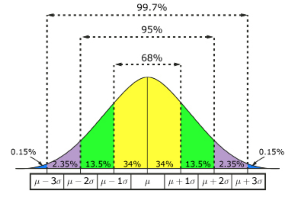
In other words, suppose that the heights of women are normally distributed with a mean height of 63.6 inches and a standard deviation of 2.5 inches. What percentage of women are taller than 68.6 inches?

If you think about it for a moment, you may realize that 68.6 is two “standard deviations” above the mean of 63.6 (because 63.6 + 2.5 + 2.5 = 68.3). That means that women who are taller will lie ABOVE the “μ+2σ” line on the normal distribution.

By looking at the graphic, you can see that there are 2.35% + 0.15% = 2.5% of women above that point – so the answer is that 2.5% of women are taller than 68.3 inches.

And that’s some basic info about the CSET Math Subtest II.

CSET Math Subtest III

Overview

Subtest III has 30 multiple-choice questions and 2 constructed-response questions.

There is one domain with specific competencies:

• Calculus
• Trigonometry
• Limits and Continuity
• Derivatives and Applications
• Integrals and Applications
• Sequences and Series

So, let’s start with Trigonometry.

Calculus: Trigonometry

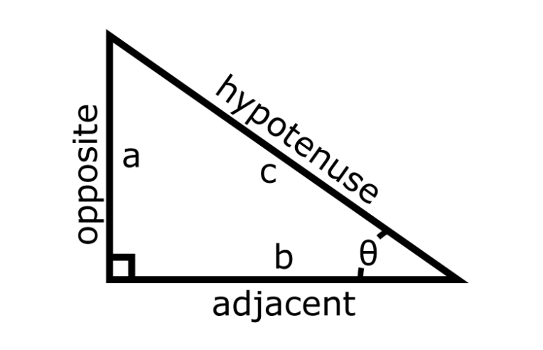
Trigonometry is the study of triangles – or, more accurately, the study of right triangles. This may make trigonometry seem rather limited in its scope, but it is among the most useful and powerful areas of mathematics, with applications in navigation, cartography, astronomy, architecture, engineering, GPS systems, and many more.

Pictured above is a right triangle with sides a and b and hypotenuse c. Also indicated is the right angle on the left and an angle θ (Theta) on the right. The sides are labeled as being “opposite” the angle θ, or “adjacent” to the angle θ.

The single most important thing you will learn in trigonometry is the word SOH-CAH-TOA.

This word is an acronym that helps you to remember the definitions of the three important trig functions: sine, cosine, and tangent, abbreviated as sin, cos, and tan.

Notice that in the reciprocal functions, cosecant and sine go together, and cosine and secant go together. This is a handy way to remember these: if one has a “co,” the other doesn’t.

Here are some other concepts to check out and study.

The Unit Circle

Trigonometry is about triangles, but it is also done in a circle. Imagine that you have a circle with a radius of length 1 . This is called a “unit circle,” and by taking an angle θ in that circle, you can visualize the trig functions in a new way:

As you can see, when you sweep the radius up to form an angle θ with the x-axis, you can create a right triangle. Now, look at the point where the blue radius intersects the circle. Since the hypotenuse has a length of 1, the cosine of that angle θ is just the x -coordinate of that point, and the sine of that angle θ is just the y-coordinate. We can use the unit circle to apply trigonometry to many things. That’s pretty cool!

Trig Identities

There are some important relationships between trig functions which we call the trig identities. The most well known of these is the Pythagorean identity :

Two other common trig identities are called the double angle and half-angle formulas. The double angle formulas for sine and cosine are:

The half-angle formulas for sine and cosine are:

And finally, we have the Ptolemy identities, also known as the sum and difference formulas:

Calculus: Limits and Continuity

The concept of the limit is one of the most important concepts in all of higher mathematics, and it is certainly the beating heart of the study of calculus. Recall from geometry that a function maps any given input x from its domain to one (and only one) output, f(x) , in its range. The idea behind limits is to think about what the output, f(x) , is approaching as x approaches a certain value.

Now, sometimes this will be fairly intuitive. Take the function f(x) = x² , for example. When x approaches 2 – that is, as x gets closer and closer to taking on the value of 2, x² approaches 4. Notably, this is still true if we restrict the domain of the function to specifically exclude x=2 . The function f(x) = x² ; x ≠ 2 is not defined when x=2 , but as x gets “close” to 2, f(x) gets “close” to 4.

Here are concepts that you may see on the test.

Basic Properties of Limits and Continuity

In the study of limits, we sometimes consider limits from only one direction. These one-sided limits are useful because they are the basis of continuity. For a function f(x) and a value a in the domain of f(x) , we can think about what happens when the function approaches that value from the left or right.

This is called a left-hand limit . This is the limit as x approaches a from the negative direction – from the left-hand side. Similarly:

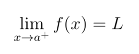
This is called a right-hand limit. This is the limit as x approaches a from the positive direction – the right-hand side.

When these two limits are equal, we say that:

And f(x) is said to be continuous at x=a .

Limits of Rational Functions

One of the most common types of problems you will see regarding limits involve the limits of rational functions. Typically, such functions will involve a discontinuity at a certain point which, if one simply evaluated the function at that point, would result in division by zero or something similarly disallowed.

One way to “remove” such a discontinuity is by factoring. For example, consider this limit:

This function is discontinuous at x=1, because “plugging in” 1 will result in division by zero; however, by factoring the numerator, we can arrive at:

Now, we have an x-1 in the numerator and denominator, which will cancel, leaving us with:

Once you reach a point where you can evaluate the function without division by zero, that value is the limit you are looking for.

Calculus: Derivatives and Applications

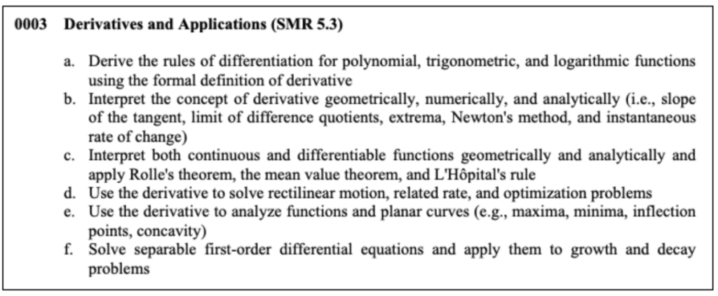
Recall from geometry that one of the things we can do with lines in the plane is figure out the slope of that line. But what about curves? To find the slope of a curve, the derivative is the answer. Derivatives are functions which describe the slope of a function at any point, but there are more important ways to think about them. The derivative is best interpreted as a rate of change , and so it has important applications in physics, astronomy, engineering, and other sciences.

For a function f(x) , its derivative is denoted:

Let’s look at some specific concepts that may come up on the test.

The basic rules for derivatives are as follows:

Power Rule

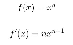
In other words, to take the derivative with respect to x, multiply x by its power, and subtract one from that power. This also gives us a useful consequence:

The derivative of x (with respect to x ) is 1.

Sum/Difference Rule

The sum and difference rule tells us that for a polynomial function, we can simply apply the power rule to each term.

Constant Rule

The derivative of a constant without the variable attached is simply zero.

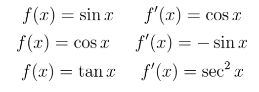
Derivatives of Trig Functions

The basic trigonometric functions have derivatives that aren’t too hard to remember:

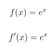
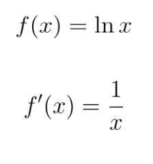
Exponential Functions and Logarithms

For the exponential function e× :

For the natural logarithm ln x:

Product Rule

To take the derivative of the product of two functions, you must use this rule:

The easiest way to remember this process is simply to talk through it: “The first times the derivative of the second, plus the derivative of the first times the second.” For example:

Quotient Rule

The quotient rule is used in rational functions.

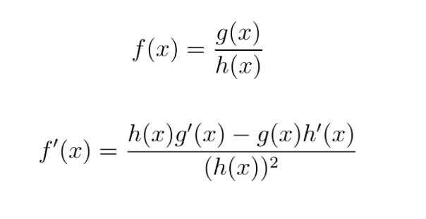
A useful mnemonic for remembering this is the poem:

Lo D-Hi, Hi D-Lo Square the bottom and there you go. In other words, the numerator is the bottom function times the derivative of the top, minus the top function times the derivative of the bottom, and then the denominator is squared.

Chain Rule

The chain rule is used for function compositions when one function is “nested” inside another. It can be tricky to recognize when it is happening, but in general, look for:

• Exponents with a variable in them, such as 32x
• Trig functions with something more than just x, such as sin(3x)
• Logarithms of more than just x, such as ln(3x 2 +9)

Here is how the chain rule works:

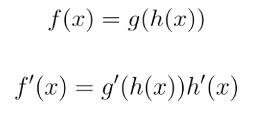
In other words, to perform the chain rule, take the derivative of the “outside” function times the derivative of the “inside” function.

For example:

Calculus: Integrals and Applications

This section tests your knowledge on antiderivatives, indefinite integrals, and definite integrals. Antiderivatives and integrals are essentially the “opposite” of differentiation, but integrals have some surprising applications in physics, engineering, and even health sciences.

Here are some specific concepts that will more than likely appear on the test.

Antiderivatives

Suppose that you know that:

Can you figure out what the original function is? By thinking about the steps you use to take a derivative, you may be able to see that the answer is:

If you have trouble seeing this, take the derivative of x 3 and see what you get. Remember the power rule, and think about it in reverse.

Think about this: what if y=x³  + 1 ?

If you differentiate this function, you still end up with:

So, we must allow for the possibility of a constant term in our original function when taking the antiderivative.

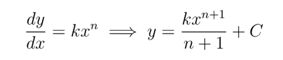
In general, to find the antiderivative of kx^n , where k is some coefficient (which could be 1), and n is some power of x , you will:

1. Add one to n.
2. Divide the whole term by n+1(the NEW power).
3. Add an arbitrary constant, C.

In notation, this is:

For example, find an antiderivative of:

Indefinite Integrals

Once you know how to find an antiderivative, you know the basics of integration. The indefinite integral of a function is the collection of all its antiderivatives . For example, the example we just did could be written this way:

…for all real values of C . The addition of the arbitrary constant makes this the collection of all antiderivatives for our function.

A few notes on notation:

• The integral sign is an elongated “S” and stands for “sum.” An integral is a limit of something called a Riemann sum.
• The Riemann sum approximates a function with a series of rectangles and “sums” up their areas. In the limit, the width of these rectangles is made arbitrarily small (so you end up with something that looks exactly like the function).
• The “dx” at the end is important – it represents the “width” of each rectangle. Don’t forget the dx!
• When using indefinite integrals, the +C is important! Don’t forget this, either.

Calculus: Sequences and Series

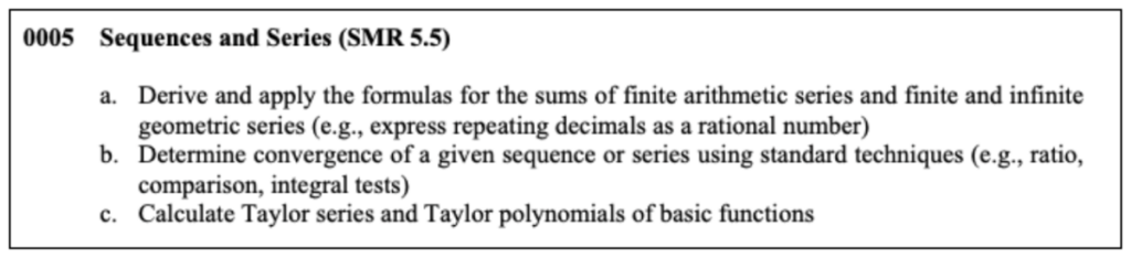
This section tests your knowledge on sequences and series of real numbers. A sequence of numbers is simply a list of numbers, in order, usually with some rule or recursion that defines how the sequence is constructed. A series , on the other hand, is the sum of the elements in a sequence.

Let’s discuss some concepts that will more than likely appear on the test.

Sequences

Sequences use the same notation as sets: {1,2,3,4,5,…} denotes the sequence of positive integers. Notice that this sequence is infinite – there is no largest positive integer, after all. Sequences may be infinite or finite.

Usually, when discussing sequences, it is important to consider the “rule” or “recursion” that will generate that sequence. For example, the sequence {3, 5, 7, 9, …}, or all the positive odd integers greater than 1, can be expressed as a recursion with a formula. To figure out what that formula is, we need a little notation first.

In a sequence, each term is denoted a n where n is its “place” in the order of the sequence. In this example, a 1 = 3, a 2 = 5, a 3 = 7, and so on. Our job is to write something general, like a n = ? to describe any arbitrary number in the sequence.

Since for the first term, n=1 , we need to begin there and ask “how can we turn a 1 into a 3?” Well, 2n+1 will do it… will that work for the rest of the entries?

It looks like we’re golden!

Here are some well-known sequences:

• Arithmetic sequence: Any sequence where the difference between each term and the next is constant. For example, in the sequence {1, 4, 7, 11, …} each term differs by 3.
• Geometric sequence: A sequence in which the next term is found by multiplying the previous term by a constant. For example, the sequence {2, 4, 8, 16, 32, 64, …} is a geometric sequence, because each term is the previous term times 2.
• Fibonacci sequence: Perhaps one of the best known sequences, the Fibonacci sequence begins witha1 = 0 and a 2 = 1 , and then a n = a n-2 + a n-1 – in other words, after the first two terms which are defined, each term is the sum of the two previous. The first few terms in the Fibonacci sequence are {0, 1, 1, 2, 3, 5, 8, 13, 21, 34, 55 …}.

Series

As mentioned, a series is the sum of all the entries in a sequence. Sometimes (and in fact, this is the case with all sequences mentioned as examples here) this sum keeps getting bigger and bigger the more terms we add, and so the sum approaches infinity – in this case, we say that the sum diverges. Somehow, however, it is possible to have a series that sums to a number. In this case, we say that a series converges .

Finite and Infinite Geometric Series

A geometric series is, not surprisingly, a series (or sum) of a geometric sequence. We often use “sigma notation” to write series, since they are sums. It looks like this:

That is, “the sum from i=1 to i=n of all the a i terms in a sequence.

Consider the finite geometric sequence:

This corresponds to the finite geometric series:

and is written in sigma notation as:

But what if we didn’t stop after that 7th term in the geometric sequence? If we consider the infinite geometric sequence, then the related geometric series would be:

and is written in sigma notation as:

To find the sum of a geometric series, use the formula:

In this formula, S n is called the partial sum – in an infinite series, we would consider the limit of this sum as it approaches infinity. The term a 1 is the first term of the sequence, and r is the common ratio between terms – to figure out what it is, simply divide a 1 by a 2 .

Importantly, if r <1, then you can use the formula:

and the series converges to a number.

Conversely, if r>1 , then the series will not converge – it will diverge to infinity.

And that’s some basic info about the CSET Math Subtest III.